Chapter 3 Cookbook -- Cool things to do with it

3.1 BLAST

Hey, everybody loves BLAST right? I mean, geez, how can get it get any easier to do comparisons between one of your sequences and every other sequence in the known world? Heck, if I was writing the code to do that it would probably take about a day and a half to complete, and the results still wouldn't be as good. But, of course, this section isn't about how cool BLAST is, since we already know that. It is about the problem with BLAST -- it can be really difficult to deal with the volume of data generated by large runs, and to automate BLAST runs in general.

Fortunately, the Biopython folks know this only too well, so they've developed lots of tools for dealing with BLAST and making things much easier. This section details how to use these tools and do useful things with 'em.

3.1.1 Running BLAST over the internet

The first step in automating BLASTing is to make everything accessable from python scripts. So, biopython contains code that allows you to run the WWW version of BLAST (http://www.ncbi.nlm.nih.gov/BLAST/) directly from your python scripts. This is very nice, especially since BLAST can be a real pain to deal with from scripts, especially with the whole BLAST queue thing and the separate results page. Keeping the BioPython code up to date with all of the changes at NCBI is hard enough!

The code to deal with the WWW version of BLAST is found in the Bio.Blast.NCBIWWW module, and the blast function. Let's say we want to BLAST info we have in a FASTA formatted file against the database. First, we need to get the info in the FASTA file. The easiest way to do this is to use the Fasta iterator to get a record. In this example, we'll just grab the first FASTA record from a file, using an Iterator (section 2.4.3 explains FASTA iterators in more detail).

from Bio import Fasta

file_for_blast = open('m_cold.fasta', 'r')
f_iterator = Fasta.Iterator(file_for_blast)

f_record = f_iterator.next()

Now that we've got the FASTA record, we are ready to blast it. The code to do the simplest possible BLAST (a simple blastn of the FASTA file against all of the non-redundant databases) is:

from Bio.Blast import NCBIWWW
b_results = NCBIWWW.blast('blastn', 'nr', f_record)

The blast function also take a number of other option arguments which are basically analogous to the different parameters you can set on the basic BLAST page (http://www.ncbi.nlm.nih.gov/blast/blast.cgi?Jform=0), but for this I'll just talk about the first few arguments, which are the most important (and are also non-optional).

The first argument is the blast program to use for the search. The options and descriptions of the programs are available at http://www.ncbi.nlm.nih.gov/BLAST/blast_program.html. The second argument specifies the databases to search against. Again, the options for this are available on the NCBI web pages at http://www.ncbi.nlm.nih.gov/BLAST/blast_databases.html.

After you have set the search options, you just need to pass in your fasta sequence as a string, which is the third argument, and you are all ready to BLAST. Biopython takes care of worrying about when the results are available, and will pause until it can get the results and return them.

Before parsing the results, it is often useful to save them into a file so that you can use them later without having to go back and re-blast everything. I find this especially useful when debugging my code that extracts info from the BLAST files, but it could also be useful just for making backups of things you've done. If you want to save the results returned, and also parse the results, we need to be careful since using handle.read() to write the results to the file will result in not having the info in the handle anymore. The best way to handle this is to first use read() to get all of the information from the handle into a string, and then deal with this string (note: using the copy module will not work, despite what was written here before (whoops!), since it is not possible to copy a handle). We can get a string with the BLAST results and write it to a file by doing:

# save the results for later, in case we want to look at it
save_file = open('my_blast.out', 'w')
blast_results = result_handle.read()
save_file.write(blast_results)
save_file.close()

After doing this, the results are in the file my_blast.out and the variable blast_results contains the blast results in a string form.

The parse function of the BLAST parser, as described in 3.1.2, takes a file-handle-like object to be parsed. We can get a handle-like object from our string of BLAST results using the python standard library module cStringIO. The following code will give us a handle we can feed directly into the parser:

import cStringIO
string_result_handle = cStringIO.StringIO(blast_results)

Now that we've got the BLAST results, we are ready to do something with them, so this leads us right into the parsing section.

3.1.2 Parsing the output from the WWW version of BLAST

The WWW version of BLAST is infamous for continually changing the output in a way that will break parsers that deal with it. Because of this, having a centralized parser in libraries such as Biopython is very important, since then you can have multiple people testing and using it and keeping it up to date. This is so much nicer than trying to keep a tool such as this running yourself.

You can get information to parse with the WWW BLAST parser in one of the two ways. The first is to grab the info using the biopython function for dealing with blast -- doing this is described in section 3.1.1. The second way is to manually do the BLAST on the NCBI site, and then save the results. In order to have your output in the right format, you need to save the final BLAST page you get (you know, the one with all of the interesting results!) as HTML (i. e. do not save as text!) to a file. The important point is that you do not have to use biopython scripts to fetch the data in order to be able to parse it.

Doing things either of these two ways, you then need to get a handle to the results. In python, a handle is just a nice general way of describing input to any info source so that the info can be retrieved using read() and readline() functions. This is the type of input the BLAST parser (and the other biopython parsers take).

If you followed the code above for interacting with BLAST through a script, then you already have blast_results, which is great for passing to a parser. If you saved the results in a file, then opening up the file with code like the following will get you what you need:

blast_results = open('my_blast_results', 'r')

Now that we've got a handle, we are ready to parse the output. The code to parse it is really quite small:

from Bio.Blast import NCBIWWW

b_parser = NCBIWWW.BlastParser()
b_record = b_parser.parse(b_results)

What this accomplishes is parsing the BLAST output into a Blast Record class. The section below on the Record class describes what is contained in this class, but in general, it has got everything you might ever want to extract from the output. Right now we'll just show an example of how to get some info out of the BLAST report, but if you want something in particular that is not described here, look at the info on the record class in detail, and take a gander into the code or automatically generated documentation -- the docstrings have lots of good info about what is stored in each piece of information.

To continue with our example, let's just print out some summary info about all hits in our blast report greater than a particular threshold. The following code does this:

E_VALUE_THRESH = 0.04

for alignment in b_record.alignments:
    for hsp in alignment.hsps:
        if hsp.expect < E_VALUE_THRESH:
            print '****Alignment****'
            print 'sequence:', alignment.title
            print 'length:', alignment.length
            print 'e value:', hsp.expect
            print hsp.query[0:75] + '...'
            print hsp.match[0:75] + '...'
            print hsp.sbjct[0:75] + '...'

This will print out summary reports like the following:

****Alignment****
sequence: >gb|AF283004.1|AF283004 Arabidopsis thaliana cold acclimation protein WCOR413-like protein
alpha form mRNA, complete cds
length: 783
e value: 0.034
tacttgttgatattggatcgaacaaactggagaaccaacatgctcacgtcacttttagtcccttacatattcctc...
||||||||| | ||||||||||| || ||||  || || |||||||| |||||| |  | |||||||| ||| ||...
tacttgttggtgttggatcgaaccaattggaagacgaatatgctcacatcacttctcattccttacatcttcttc...

Basically, you can do anything you want to with the info in the BLAST report once you have parsed it. This will, of course, depend on what you want to use it for, but hopefully this helps you get started on doing what you need to do!

3.1.3 The BLAST record class

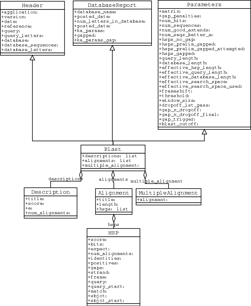
An important consideration for extracting information from a BLAST report is the type of objects that the information is stored in. In Biopython, the parsers return Record objects, either Blast or PSIBlast depending on what you are parsing. These objects are defined in Bio.Blast.Record and are quite complete.

Here are my attempts at UML class diagrams for the Blast and PSIBlast record classes. If you are good at UML and see mistakes/improvements that can be made, please let me know. The Blast class diagram is shown in Figure 3.1.3.

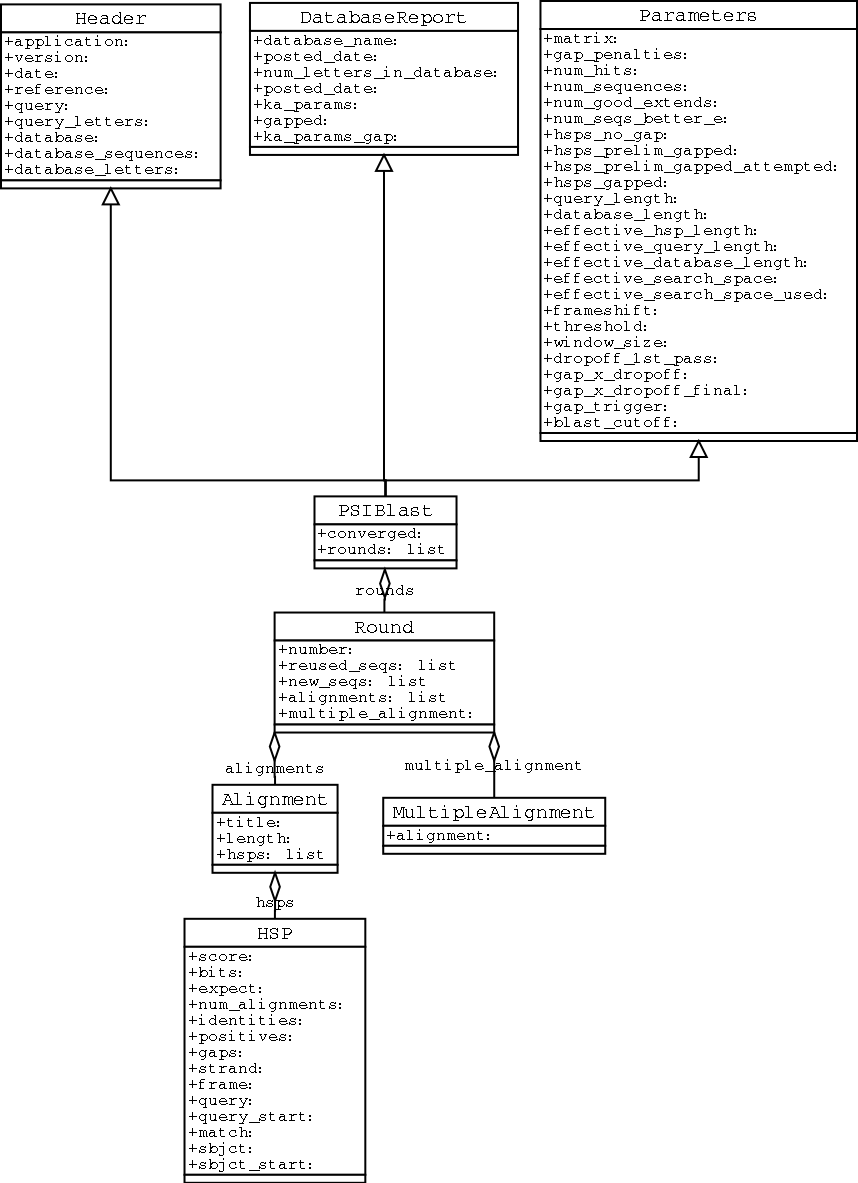
The PSIBlast record object is similar, but has support for the rounds that are used in the iteration steps of PSIBlast. The class diagram for PSIBlast is shown in Figure 3.1.3.

3.1.4 Running BLAST locally

If you want to make your own database to search for sequences against, then local BLAST is definately the way you want to go. As with online BLAST, biopython provides lots of nice code to make you able to call local BLAST executables from your scripts, and have full access to the many command line options that these executables provide. You can obtain local BLAST precompiled for a number of platforms at ftp://ncbi.nlm.nih.gov/blast/executables/, or can compile it yourself in the NCBI toolbox (ftp://ncbi.nlm.nih.gov/toolbox/).

The code for dealing with local BLAST is found in Bio.Blast.NCBIStandalone, specifically in the functions blastall and blastpgp, which correspond with the BLAST executables that their names imply.

Let's use these functions to run a blastall against a local database and return the results. First, we want to set up the paths to everything that we'll need to do the blast. What we need to know is the path to the database (which should have been prepared using formatdb) to search against, the path to the file we want to search, and the path to the blastall executable.

import os

my_blast_db = os.path.join(os.getcwd(), 'at-est', 'a_cds-10-7.fasta')
my_blast_file = os.path.join(os.getcwd(), 'at-est', 'test_blast',
                             'sorghum_est-test.fasta')
my_blast_exe = os.path.join(os.getcwd(), 'blast', 'blastall')

Now that we've got that all set, we are ready to run the blast and collect the results. We can do this with two lines:

from Bio.Blast import NCBIStandalone

blast_out, error_info = NCBIStandalone.blastall(my_blast_exe, 'blastn',
                                                my_blast_db, my_blast_file)

Note that the biopython interfaces to local blast programs returns two values. The first is a handle to the blast output, which is ready to either be saved or passed to a parser. The second is the possible error output generated by the blast command.

The error info can be hard to deal with, because if you try to do a error_info.read() and there was no error info returned, then the read() call will block and not return, locking your script. In my opinion, the best way to deal with the error is only to print it out if you are not getting blast_out results to be parsed, but otherwise to leave it alone.

If you are interested in saving your results to a file before parsing them, see the section on WWW blast above for some info on how to use the copy module to do this.

Well, now that you've got output, we should start parsing them, so read on to learn about parsing local BLAST output.

3.1.5 Parsing BLAST output from local BLAST

Since the output generated by local BLAST is different than that generated by the web-based BLAST, we use the parsers located in Bio.Blast.NCBIStandalone to parse and deal with the results.

As with WWW blast (see the info on this above) we need to have a handle object that we can pass to the parser. The handle must implement the readline() method and do this properly. The common ways to get such a handle are to either use the provided blastall or blastpgp functions to run the local blast, or to run a local blast via the commandline, and then do something like the following:

blast_out = open('my_file_of_blast_output', 'r')

So, as with WWW blast, there is no need to use the biopython convenience functions if you don't want to.

Well, now that we've got a handle (which we'll call blast_out), we are ready to parse it. This can be done with the following code:

from Bio.Blast import NCBIStandalone

b_parser = NCBIStandalone.BlastParser()
b_record = b_parser.parse(blast_out)

This will parse the BLAST report into a Blast Record class (either a Blast or a PSIBlast record, depending on what you are parsing) so that you can extract the information from it. In our case, let's just use print out a quick summary of all of the alignments greater than some threshold value.

E_VALUE_THRESH = 0.04
for alignment in b_record.alignments:
    for hsp in alignment.hsps:
        if hsp.expect < E_VALUE_THRESH:
            print '****Alignment****'
            print 'sequence:', alignment.title
            print 'length:', alignment.length
            print 'e value:', hsp.expect
            print hsp.query[0:75] + '...'
            print hsp.match[0:75] + '...'
            print hsp.sbjct[0:75] + '...'

If you also read the section on parsing BLAST from the WWW version, you'll notice that the above code is identical to what is found in that section. Once you parse something into a record class you can deal with it independent of the format of the original BLAST info you were parsing. Pretty snazzy!

Sure, parsing one record is great, but I've got a BLAST file with tons of records -- how can I parse them all? Well, fear not, the answer lies in the very next section.

3.1.6 Parsing a file full of BLAST runs

Of course, local blast is cool because you can run a whole bunch of sequences against a database and get back a nice report on all of it. So, biopython definately has facilities to make it easy to parse humungous files without memory problems.

We can do this using the blast iterator. To set up an iterator, we first set up a parser, to parse our blast reports in Blast Record objects:

from Bio.Blast import NCBIStandalone

b_parser = NCBIStandalone.BlastParser()

Then we will assume we have a handle to a bunch of blast records, which we'll call blast_out. Getting a handle is described in full detail above in the blast parsing sections.

Now that we've got a parser and a handle, we are ready to set up the iterator with the following command:

b_iterator = NCBIStandalone.Iterator(blast_out, b_parser)

The second option, the parser, is optional. If we don't supply a parser, then the iterator will just return the raw BLAST reports one at a time.

Now that we've got an iterator, we start retrieving blast records (generated by our parser) using next():

b_record = b_iterator.next()

Each call to next will return a new record that we can deal with. Now we can iterate through this records and generate our old favorite, a nice little blast report:

while 1:
    b_record = b_iterator.next()

    if b_record is None:
        break

    E_VALUE_THRESH = 0.04
    for alignment in b_record.alignments:
        for hsp in alignment.hsps:
            if hsp.expect < E_VALUE_THRESH:
                print '****Alignment****'
                print 'sequence:', alignment.title
                print 'length:', alignment.length
                print 'e value:', hsp.expect

                if len(hsp.query) > 75:
                    dots = '...'
                else:
                    dots = ''
                
                print hsp.query[0:75] + dots
                print hsp.match[0:75] + dots
                print hsp.sbjct[0:75] + dots

Notice that b_iterator.next() will return None when it runs out of records to parse, so it is easy to iterate through the entire file with a while loop that checks for the existance of a record.

The iterator allows you to deal with huge blast records without any memory problems, since things are read in one at a time. I have parsed tremendously huge files without any problems using this.

3.1.7 Finding a bad record somewhere in a huge file

One really ugly problem that happens to me is that I'll be parsing a huge blast file for a while, and the parser will bomb out with a SyntaxError. This is a serious problem, since you can't tell if the SyntaxError is due to a parser problem, or a problem with the BLAST. To make it even worse, you have no idea where the parse failed, so you can't just ignore the error, since this could be ignoring an important data point.

We used to have to make a little script to get around this problem, but the Bio.Blast module now includes a BlastErrorParser which really helps make this easier. The BlastErrorParser works very similar to the regular BlastParser, but it adds an extra layer of work by catching SyntaxErrors that are generated by the parser, and attempting to diagnose the errors.

Let's take a look at using this parser -- first we define the file we are going to parse and the file to write the problem reports to:

import os
 
b_file = os.path.join(os.getcwd(), 'blast_out', 'big_blast.out')
error_file = os.path.join(os.getcwd(), 'blast_out', 'big_blast.problems')

Now we want to get a BlastErrorParser:

from Bio.Blast import NCBIStandalone

error_handle = open(error_file, 'w')

b_error_parser = NCBIStandalone.BlastErrorParser(error_handle)

Notice that the parser take an optional argument of a handle. If a handle is passed, then the parser will write any blast records which generate a SyntaxError to this handle. Otherwise, these records will not be recorded.

Now we can use the BlastErrorParser just like a regular blast parser. Specifically, we might want to make an iterator that goes through our blast records one at a time and parses them with the error parser:

blast_out = open(b_file)
iterator = NCBIStandalone.Iterator(blast_out, b_error_parser)

Just like before, we can read these records one a time with, but now we can catch and deal with errors that are due to problems with Blast (and not with the parser itself):

try:
    next_record = iterator.next()
except NCBIStandalone.LowQualityBlastError, info:
    print "LowQualityBlastError detected in id %s" % info[1]

Right now the BlastErrorParser can generate the following errors:

SyntaxError -- This is the same error generated by the regular BlastParser, and is due to the parser not being able to parse a specific file. This is normally either due to a bug in the parser, or some kind of descrepency between the version of BLAST you are using and the versions the parser is able to handle.
LowQualityBlastError -- When BLASTing a sequence that is of really bad quality (for example, a short sequence that is basically a stretch of one nucleotide), it seems that Blast ends up masking out the entire sequence and ending up with nothing to parse. In this case it will produce a truncated report that causes the parser to generate a SyntaxError. LowQualityBlastError is reported in these cases. This error returns an info item with the following information:
- item[0] -- The error message
- item[1] -- The id of the input record that caused the error. This is really useful if you want to record all of the records that are causing problems.

As mentioned, with each error generated, the BlastErrorParser will write the offending record to the specified error_handle. You can then go ahead and look and these and deal with them as you see fit. Either you will be able to debug the parser with a single blast report, or will find out problems in your blast runs. Either way, it will definately be a useful experience!

Hopefully the BlastErrorParser will make it much easier to debug and deal with large Blast files.

3.1.8 Dealing with PSIBlast

We should write some stuff to make it easier to deal directly with PSIBlast from scripts (i. e. output the align file in the proper format from an alignment). I need to look at PSIBlast more and come up with some good ways of going this...

3.2 SWISS-PROT

3.2.1 Retrieving a SWISS-PROT record

SwissProt (http://www.expasy.ch/sprot/sprot-top.html) is a handcurated database of protein sequences. Let's look at how we connect with it from a script and parse SwissProt formatted results.

First, we need to retrieve some results to parse. Let's say we are looking at chalcone synthases for Orchids (see section 2.3 for some justification for looking for interesting things about orchids). Chalcone synthase is involved in flavanoid biosynthesis in plants, and flavanoids make lots of cool things like pigment colors and UV protectants.

If you do a search on SwissProt, you can find three orchid proteins for Chalcone Synthase, id numbers O23729, O23730, O23731. Now, let's write a script which grabs these, and parses out some interesting information.

First, we grab the records, using the get_sprot_raw() function of Bio.WWW.Expasy. This function is very nice since you can feed it an id and get back a raw text record (no html to mess with!). As we get the three records we are interested in, we'll just put them together into one big string, which we'll then use for parsing. The following code accomplishes what I just wrote:

from Bio.WWW import ExPASy

ids = ['O23729', 'O23730', 'O23731']

all_results = ''
for id in ids:
    results = ExPASy.get_sprot_raw(id)
    all_results = all_results + results.read()

Now that we've got the results, we are ready to parse them into interesting information. As with most parsers, we set up an iterator and parser. The parser we use here parses the SwissProt files into a Record object where the interesting features are attributes:

from Bio.SwissProt import SProt
from Bio import File

s_parser = SProt.RecordParser()
s_iterator = SProt.Iterator(File.StringHandle(all_results), s_parser)

Note that we convert all_results, which is a string, into a handle before passing it. The iterator requires a handle to be passed so that it can read in everything one line at a time. The Bio.File module has a nice StringHandle, which conveniently will convert a string into a handle. Very nice! Now we are ready to start extracting information.

To get out the information, we'll go through everything record by record using the iterator. For each record, we'll just print out some summary information:

while 1:
    cur_record = s_iterator.next()

    if cur_record is None:
        break

    print "description:", cur_record.description
    for ref in cur_record.references:
        print "authors:", ref.authors
        print "title:", ref.title

    print "classification:", cur_record.organism_classification
    print

This prints out a summary like the following:

description: CHALCONE SYNTHASE 8 (EC 2.3.1.74) (NARINGENIN-CHALCONE SYNTHASE 8)
authors: Liew C.F., Lim S.H., Loh C.S., Goh C.J.;
title: "Molecular cloning and sequence analysis of chalcone synthase cDNAs of
Bromheadia finlaysoniana.";
classification: ['Eukaryota', 'Viridiplantae', 'Embryophyta', 'Tracheophyta', 
'Spermatophyta', 'Magnoliophyta', 'Liliopsida', 'Asparagales', 'Orchidaceae', 
'Bromheadia']

It is equally easy to extract any kind of information you'd like from SwissProt records.

3.3 PubMed

3.3.1 Sending a query to PubMed

If you are in the Medical field or interested in human issues (and many times even if you are not!), PubMed (http://www.ncbi.nlm.nih.gov/PubMed/) is an excellent source of all kinds of goodies. So like other things, we'd like to be able to grab information from it and use it in python scripts.

Querying PubMed using Biopython is extremely painless. To get all of the article ids for articles having to do with orchids, we only need the following three lines of code:

from Bio.Medline import PubMed

search_term = 'orchid'
orchid_ids = PubMed.search_for(search_term)

This returns a python list containing all of the orchid ids

['11070358', '11064040', '11028023', '10947239', '10938351', '10936520', 
'10905611', '10899814', '10856762', '10854740', '10758893', '10716342', 
...

With this list of ids we are ready to start retrieving the records, so follow on ahead to the next section.

3.3.2 Retrieving a PubMed record

The previous section described how to get a bunch of article ids. Now that we've got them, we obviously want to get the corresponding Medline records and extract the information from them.

The interface for retrieving records from PubMed should be very intuitive to python programmers -- it models a python dictionary. To set up this interface, we need to set up a parser that will parse the results that we retrieve. The following lines of code get everything set up:

from Bio.Medline import PubMed
from Bio import Medline

rec_parser = Medline.RecordParser()
medline_dict = PubMed.Dictionary(parser = rec_parser)

What we've done is create a dictionary like object medline_dict. To get an article we access it like medline_dict[id_to_get]. What this does is connect with PubMed, get the article you ask for, parse it into a record object, and return it. Very cool!

Now let's look at how to use this nice dictionary to print out some information about some ids. We just need to loop through our ids (orchid_ids from the previous section) and print out the information we are interested in:

for id in orchid_ids[0:5]:
    cur_record = medline_dict[id]
    print 'title:', string.rstrip(cur_record.title)
    print 'authors:', cur_record.authors
    print 'source:', string.strip(cur_record.source)
    print

The output for this looks like:

title: Sex pheromone mimicry in the early spider orchid (ophrys sphegodes):
patterns of hydrocarbons as the key mechanism for pollination by sexual
deception [In Process Citation]
authors: ['Schiestl FP', 'Ayasse M', 'Paulus HF', 'Lofstedt C', 'Hansson BS', 
'Ibarra F', 'Francke W']
source: J Comp Physiol [A] 2000 Jun;186(6):567-74

Especially interesting to note is the list of authors, which is returned as a standard python list. This makes it easy to manipulate and search using standard python tools. For instance, we could loop through a whole bunch of entries searching for a particular author with code like the following:

search_author = 'Waits T'

for id in our_id_list:
    cur_record = medline_dict[id]
    
    if search_author in cur_record.authors:
        print "Author %s found: %s" % (search_author,
                                       string.strip(cur_record.source))

The PubMed and Medline interfaces are very mature and nice to work with -- hopefully this section gave you an idea of the power of the interfaces and how they can be used.

3.4 GenBank

The GenBank record format is a very popular method of holding information about sequences, sequence features, and other associated sequence information. The format is a good way to get information from the NCBI databases at http://www.ncbi.nlm.nih.gov/.

3.4.1 Retrieving GenBank entries from NCBI

One very nice feature of the GenBank libraries is the ability to automate retrieval of entries from GenBank. This is very convenient for creating scripts that automate a lot of your daily work. In this example we'll show how to query the NCBI databases, and to retrieve the records from the query.

First, we want to make a query and find out the ids of the records to retrieve. Here we'll do a quick search for Opuntia, my favorite organism (since I work on it). We can do quick search and get back the GIs (GenBank identifiers) for all of the corresponding records:

from Bio import GenBank

gi_list = GenBank.search_for("Opuntia AND rpl16")

gi_list will be a list of all of the GenBank identifiers that match our query:

['6273291', '6273290', '6273289', '6273287', '6273286', '6273285', '6273284']

Now that we've got the GIs, we can use these to access the NCBI database through a dictionary interface. For instance, to retrieve the information for the first GI, we'll first have to create a dictionary that accesses NCBI:

ncbi_dict = GenBank.NCBIDictionary()

Now that we've got this, we do the retrieval:

gb_record = ncbi_dict[gi_list[0]]

In this case, gb_record will be GenBank formatted record:

LOCUS       AF191665      902 bp    DNA             PLN       07-NOV-1999
DEFINITION  Opuntia marenae rpl16 gene; chloroplast gene for chloroplast
            product, partial intron sequence.
ACCESSION   AF191665
VERSION     AF191665.1  GI:6273291
...

In this case, we are just getting the raw records. We can also pass these records directly into a parser and return the parsed record. For instance, if we wanted to get back SeqRecord objects with the GenBank file parsed into SeqFeature objects we would need to create the dictionary with the GenBank FeatureParser:

record_parser = GenBank.FeatureParser()
ncbi_dict = GenBank.NCBIDictionary(parser = record_parser)

Now retrieving a record will give you a SeqRecord object instead of the raw record:

>>> gb_seqrecord = ncbi_dict[gi_list[0]]
>>> print gb_seqrecord
<Bio.SeqRecord.SeqRecord instance at 0x102f9404>

For more information of formats you can parse GenBank records into, please see section 3.4.2.

Using these automated query retrieval functionality is a big plus over doing things by hand. Additionally, the retrieval has nice built in features like a time-delay, which will prevent NCBI from getting mad at you and blocking your access.

3.4.2 Parsing GenBank records

While GenBank files are nice and have lots of information, at the same time you probably only want to extract a small amount of that information at a time. The key to doing this is parsing out the information. Biopython provides GenBank parsers which help you accomplish this task. Right now the GenBank module provides the following parsers:

RecordParser -- This parses the raw record into a GenBank specific Record object. This object models the information in a raw record very closely, so this is good to use if you are just interested in GenBank records themselves.
FeatureParser -- This parses the raw record in a SeqRecord object with all of the feature table information represented in SeqFeatures (see section 3.7 for more info on these objects). This is best to use if you are interested in getting things in a more standard format.

Either way you chose to go, the most common usage of these will be creating an iterator and parsing through a file on GenBank records. Doing this is very similar to how things are done in other formats, as the following code demonstrates:

from Bio import GenBank

gb_file = "my_file.gb"
gb_handle = open(gb_file, 'r')

feature_parser = GenBank.FeatureParser()

gb_iterator = GenBank.Iterator(gb_handle, feature_parser)

while 1:
   cur_record = gb_iterator.next()

   if cur_record is None:
       break

   # now do something with the record
   print cur_record.seq

This just iterates over a GenBank file, parsing it into SeqRecord and SeqFeature objects, and prints out the Seq objects representing the sequences in the record.

As with other formats, you have lots of tools for dealing with GenBank records. This should make it possible to do whatever you need to with GenBank.

3.4.3 Making your very own GenBank database

One very cool thing that you can do is set up your own personal GenBank database and access it like a dictionary (this can be extra cool because you can also allow access to these local databases over a network using BioCorba -- see the BioCorba documentation for more information).

Making a local database first involves creating an index file, which will allow quick access to any record in the file. To do this, we use the index file function:

>>> from Bio import GenBank
>>> dict_file = 'cor6_6.gb'
>>> index_file = 'cor6_6.idx'
>>> GenBank.index_file(dict_file, index_file)

This will create the file my_index_file.idx. Now, we can use this index to create a dictionary object that allows individual access to every record. Like the Iterator and NCBIDictionary interfaces, we can either get back raw records, or we can pass the dictionary a parser that will parse the records before returning them. In this case, we pass a FeatureParser so that when we get a record, then we retrieve a SeqRecord object.

Setting up the dictionary is as easy as one line:

>>> gb_dict = GenBank.Dictionary(index_file, GenBank.FeatureParser())

Now we can deal with this like a dictionary. For instance:

>>> len(gb_dict)
7
>>> gb_dict.keys()
['L31939', 'AJ237582', 'X62281', 'AF297471', 'M81224', 'X55053']

Finally, we retrieve objects using subscripting:

>>> gb_dict['AJ237582']
<Bio.SeqRecord.SeqRecord instance at 0x102fdd8c>

3.5 Dealing with alignments

It is often very useful to be able to align particular sequences. I do this quite often to get a quick and dirty idea of relationships between sequences. Consequently, it is very nice to be able to quickly write up a python script that does an alignment and gives you back objects that are easy to work with. The alignment related code in Biopython is meant to allow python-level access to alignment programs so that you can run alignments quickly from within scripts.

3.5.1 Clustalw

Clustalx (http://www-igbmc.u-strasbg.fr/BioInfo/ClustalX/Top.html) is a very nice program for doing multiple alignments. Biopython offers access to alignments in clustal format (these normally have a *.aln extension) that are produced by Clustalx. It also offers access to clustalw, which the is command line version of clustalx.

The first step in interacting with clustalw is to set up a command line you want to pass to the program. Clustalw has a ton of command line options, and if you set a lot of parameters, you can end up typing in a huge ol' command line quite a bit. This command line class models the command line by making all of the options be attributes of the class that can be set. A few convenience functions also exist to set certain parameters, so that some error checking on the parameters can be done.

To create a command line object to do a clustalw multiple alignment we do the following:

import os
from Align.Clustalw import MultipleAlignCL

cline = MultipleAlignCL(os.path.join(os.curdir, 'opuntia.fasta'))
cline.set_output('test.aln')

First we import the MultipleAlignCL object, which models running a multiple alignment from clustalw. We then initialize the command line, with a single argument of the fasta file that we are going to be using for the alignment. The initialization function also takes an optional second argument which specifies the location of the clustalw executable. By default, the commandline will just be invoked with 'clustalw,' assuming that you've got it somewhere on your PATH.

The second argument sets the output to go to the file test.aln. The MultipleAlignCL object also has numerous other parameters to specify things like output format, gap costs, etc.

We can look at the command line we have generated by invoking the __str__ member attribute of the MultipleAlignCL class. This is done by calling str(cline) or simple by printing out the command line with print cline. In this case, doing this would give the following output:

clustalw ./opuntia.fasta -OUTFILE=test.aln

Now that we've set up a simple command line, we now want to run the commandline and collect the results so we can deal with them. This can be done using the do_alignment function of Clustalw as follows:

from Bio import Clustalw

alignment = Clustalw.do_alignment(cline)

What happens when you run this if that Biopython executes your command line and runs clustalw with the given parameters. It then grabs the output, and if it is in a format that Biopython can parse (currently only clustal format), then it will parse the results and return them as an alignment object of the appropriate type. So in this case since we are getting results in the default clustal format, the returned alignment object will be a ClustalAlignment type.

Once we've got this alignment, we can do some interesting things with it such as get seq_record objects for all of the sequences involved in the alignment:

all_records = alignment.get_all_seqs()

print 'description:', all_records[0].description
print 'sequence:', all_records[0].seq

This prints out the description and sequence object for the first sequence in the alignment:

description: gi|6273285|gb|AF191659.1|AF191
sequence: Seq('TATACATTAAAGAAGGGGGATGCGGATAAATGGAAAGGCGAAAGAAAGAAAAAAATGAAT 
...', IUPACAmbiguousDNA())

You can also calculate the maximum length of the alignment with:

length = alignment.get_alignment_length()

Finally, to write out the alignment object in the original format, we just need to access the __str__ function. So doing a print alignment gives:

CLUSTAL X (1.81) multiple sequence alignment


gi|6273285|gb|AF191659.1|AF191      TATACATTAAAGAAGGGGGATGCGGATAAATGGAAAGGCGAAAGAAAGAA
gi|6273284|gb|AF191658.1|AF191      TATACATTAAAGAAGGGGGATGCGGATAAATGGAAAGGCGAAAGAAAGAA
...

This makes it easy to write your alignment back into a file with all of the original info intact.

If you want to do more interesting things with an alignment, the best thing to do is to pass the alignment to an alignment information generating object, such as the SummaryInfo object, described in section 3.5.2.

3.5.2 Calculating summary information

Once you have an alignment, you are very likely going to want to find out information about it. Instead of trying to have all of the functions that can generate information about an alignment in the alignment object itself, we've tried to separate out the functionality into separate classes, which act on the alignment.

Getting ready to calculate summary information about an object is quick to do. Let's say we've got an alignment object called alignment. All we need to do to get an object that will calculate summary information is:

from Bio.Align import AlignInfo
summary_align = AlignInfo.SummaryInfo(alignment)

The summary_align object is very useful, and will do the following neat things for you:

Calculate a quick consensus sequence -- see section 3.5.3
Get a position specific score matrix for the alignment -- see section 3.5.4
Calculate the information content for the alignment -- see section 3.5.5
Generate information on substitutions in the alignment -- section 3.6 details using this to generate a substitution matrix.

3.5.3 Calculating a quick consensus sequence

The SummaryInfo object, described in section 3.5.2, provides functionality to calculate a quick consensus of an alignment. Assuming we've got a SummaryInfo object called summary_align we can calculate a consensus by doing:

consensus = summary_align.dumb_consensus()

As the name suggests, this is a really simple consensus calculator, and will just add up all of the residues at each point in the consensus, and if the most common value is higher than some threshold value (the default is .3) will add the common residue to the consensus. If it doesn't reach the threshold, it adds an ambiguity character to the consensus. The returned consensus object is Seq object whose alphabet is inferred from the alphabets of the sequences making up the consensus. So doing a print consensus would give:

consensus Seq('TATACATNAAAGNAGGGGGATGCGGATAAATGGAAAGGCGAAAGAAAGAAAAAAATGAAT 
...', IUPACAmbiguousDNA())

You can adjust how dumb_consensus works by passing optional parameters:

the threshold: This is the threshold specifying how common a particular residue has to be at a position before it is added. The default is .7.
the ambiguous character: This is the ambiguity character to use. The default is 'N'.
the consensus alphabet: This is the alphabet to use for the consensus sequence. If an alphabet is not specified than we will try to guess the alphabet based on the alphabets of the sequences in the alignment.

3.5.4 Position Specific Score Matrices

Position specific score matrices (PSSMs) summarize the alignment information in a different way than a consensus, and may be useful for different tasks. Basically, a PSSM is a count matrix. For each column in the alignment, the number of each alphabet letters is counted and totaled. The totals are displayed relative to some representative sequence along the left axis. This sequence may be the consesus sequence, but can also be any sequence in the alignment. For instance for the alignment:

GTATC
AT--C
CTGTC

the PSSM for this alignment is:

Let's assume we've got an alignment object called c_align. To get a PSSM with the consensus sequence along the side we first get a summary object and calculate the consensus sequence:

summary_align = AlignInfo.SummaryInfo(c_align)
consensus = summary_align.dumb_consensus()

Now, we want to make the PSSM, but ignore any N ambiguity residues when calculating this:

my_pssm = summary_align.pos_specific_score_matrix(consensus,
                                                  chars_to_ignore = ['N'])

Two notes should be made about this:

To maintain strictness with the alphabets, you can only include characters along the top of the PSSM that are in the alphabet of the alignment object. Gaps are not included along the top axis of the PSSM.
The sequence passed to be displayed along the left side of the axis does not need to be the consensus. For instance, if you wanted to display the second sequence in the alignment along this axis, you would need to do:
```
second_seq = alignment.get_seq_by_num(1)
my_pssm = summary_align.pos_specific_score_matrix(second_seq
                                                  chars_to_ignore = ['N'])
```

The command above returns a PSSM object. To print out the PSSM as we showed above, we simply need to do a print my_pssm, which gives:

    A   C   G   T
T  0.0 0.0 0.0 7.0
A  7.0 0.0 0.0 0.0
T  0.0 0.0 0.0 7.0
A  7.0 0.0 0.0 0.0
C  0.0 7.0 0.0 0.0
A  7.0 0.0 0.0 0.0
T  0.0 0.0 0.0 7.0
T  1.0 0.0 0.0 6.0
...

You can access any element of the PSSM by subscripting like your_pssm[sequence_number][residue_count_name]. For instance, to get the counts for the 'A' residue in the second element of the above PSSM you would do:

>>> print my_pssm[1]['A']
7.0

The structure of the PSSM class hopefully makes it easy both to access elements and to pretty print the matrix.

3.5.5 Information Content

A potentially useful measure of evolutionary conservation is the information ceontent of a sequence.

A useful introduction to information theory targetted towards molecular biologists can be found at http://www.lecb.ncifcrf.gov/~toms/paper/primer/. For our purposes, we will be looking at the information content of a consesus sequence, or a portion of a consensus sequence. We calculate information content at a particular column in a multiple sequence alignment using the following formula:

IC_j =

N_a

i=1

P_ij * log(

P_ij

Q_i

)

where:

IC_j -- The information content for the jth column in an alignment.
N_a -- The number of letters in the alphabet.
P_ij -- The frequency of a particular letter in the column (i. e. if G occured 3 out of 6 times in an aligment column, this would be 0.5)
Q_i -- The expected frequency of a letter. This is an optional argument, usage of which is left at the user's discretion. By default, it is automatically assigned to 0.05 for a protein alphabet, and 0.25 for a nucleic acid alphabet. This is for geting the information content without any assumption of prior distribtions. When assuming priors, or when using a non-standard alphabet, user should supply the values for Q_i.

Well, now that we have an idea what information content is being calculated in Biopython, let's look at how to get it for a particular region of the alignment.

First, we need to use our alignment to get a alignment summary object, which we'll assume is called summary_align (see section 3.5.2) for instructions on how to get this. Once we've got this object, calculating the information content for a region is as easy as:

info_content = summary_align.information_content(5, 30, 
                                                 chars_to_ignore = ['N'])

Wow, that was much easier then the formula above made it look! The variable info_content now contains a float value specifying the information content over the specified region (from 5 to 30 of the alignment). We specifically ignore the ambiguity residue 'N' when calculating the information content, since this value is not included in our alphabet (so we shouldn't be interested in looking at it!).

As mentioned above, we can also calculate relative information content by supplying the expected frequencies:

expect_freq = {
    'A' : .3,
    'G' : .2,
    'T' : .3,
    'C' : .2}

The expected should not be passed as a raw dictionary, but instead by passed as a SubsMat.FreqTable object (see section 4.4.2 for more information about FreqTables). The FreqTable object provides a standard for associating the dictionary with an Alphabet, similar to how the Biopython Seq class works.

To create a FreqTable object, from the frequency dictionary you just need to do:

from Bio.Alphabet import IUPAC
from Bio.SubsMat import FreqTable

e_freq_table = FreqTable.FreqTable(expect_freq, FreqTable.FREQ,
                                   IUPAC.unambigous_dna)

Now that we've got that, calculating the relative information content for our region of the alignment is as simple as:

info_content = summary_align.information_content(5, 30,
                                                 e_freq_table = e_freq_table,
                                                 chars_to_ignore = ['N'])

Now, info_content will contain the relative information content over the region in relation to the expected frequencies.

The value return is calculated using base 2 as the logarithm base in the formula above. You can modify this by passing the parameter log_base as the base you want:

info_content = summary_align.information_content(5, 30, log_base = 10
                                                 chars_to_ignore = ['N'])

Well, now you are ready to calculate information content. If you want to try applying this to some real life problems, it would probably be best to dig into the literature on information content to get an idea of how it is used. Hopefully your digging won't reveal any mistakes made in coding this function!

3.5.6 Translating between Alignment formats

One thing that you always end up having to do is convert between different formats. Biopython does this using a FormatConverter class for alignment objects. First, let's say we have just parsed an alignment from clustal format into a ClustalAlignment object:

import os
from Bio import Clustalw

alignment = Clustalw.parse_file(os.path.join(os.curdir, 'test.aln'))

Now, let's convert this alignment into FASTA format. First, we create a converter object:

from Bio.Align.FormatConvert import FormatConverter

converter = FormatConverter(alignment)

We pass the converter the alignment that we want to convert. Now, to get this in FASTA alignment format, we simply do the following:

fasta_align = converter.to_fasta()

Looking at the newly created fasta_align object using print fasta_align gives:

>gi|6273285|gb|AF191659.1|AF191
TATACATTAAAGAAGGGGGATGCGGATAAATGGAAAGGCGAAAGAAAGAATATATA----
------ATATATTTCAAATTTCCTTATATACCCAAATATAAAAATATCTAATAAATTAGA
...

The conversion process will, of course, lose information specific to a particular alignment format. Howerver, most of the basic information about the alignment will be retained.

As more formats are added the converter will be beefed up to read and write all of these different formats.

3.6 Substitution Matrices

Substitution matrices are an extremely important part of everyday bioinformatics work. They provide the scoring terms for classifying how likely two different residues are to substitute for each other. This is essential in doing sequence comparisons. The book ``Biological Sequence Analysis'' by Durbin et al. provides a really nice introduction to Substitution Matrices and their uses. Some famous substitution matrices are the PAM and BLOSUM series of matrices.

Biopython provides a ton of common substitution matrices, and also provides functionality for creating your own substitution matrices.

3.6.1 Using common substitution matrices

3.6.2 Creating your own substitution matrix from an alignment

A very cool thing that you can do easily with the substitution matrix classes is to create your own substitution matrix from an alignment. In practice, this is normally done with protein alignments. In this example, we'll first get a biopython alignment object and then get a summary object to calculate info about the alignment:

from Bio import Clustalw
from Bio.Alphabet import IUPAC
from Bio.Align import AlignInfo

# get an alignment object from a Clustalw alignment output
c_align = Clustalw.parse_file('protein.aln', IUPAC.protein)
summary_align = AlignInfo.SummaryInfo(c_align)

Sections 3.5.1 and 3.5.2 contain more information on doing this.

Now that we've got our summary_align object, we want to use it to find out the number of times different residues substitute for each other. To make the example more readable, we'll focus on only amino acids with polar charged side chains. Luckily, this can be done easily when generating a replacement dictionary, by passing in all of the characters that should be ignored. Thus we'll create a dictionary of replacements for only charged polar amino acids using:

replace_info = summary_align.replacement_dictionary(["G", "A", "V", "L", "I",
                                                     "M", "P", "F", "W", "S",
                                                     "T", "N", "Q", "Y", "C"])

This information about amino acid replacements is represented as a python dictionary which will look something like:

{('R', 'R'): 2079.0, ('R', 'H'): 17.0, ('R', 'K'): 103.0, ('R', 'E'): 2.0, 
('R', 'D'): 2.0, ('H', 'R'): 0, ('D', 'H'): 15.0, ('K', 'K'): 3218.0, 
('K', 'H'): 24.0, ('H', 'K'): 8.0, ('E', 'H'): 15.0, ('H', 'H'): 1235.0, 
('H', 'E'): 18.0, ('H', 'D'): 0, ('K', 'D'): 0, ('K', 'E'): 9.0, 
('D', 'R'): 48.0, ('E', 'R'): 2.0, ('D', 'K'): 1.0, ('E', 'K'): 45.0, 
('K', 'R'): 130.0, ('E', 'D'): 241.0, ('E', 'E'): 3305.0, 
('D', 'E'): 270.0, ('D', 'D'): 2360.0}

This information gives us our accepted number of replacements, or how often we expect different things to substitute for each other. It turns out, amazingly enough, that this is all of the information we need to go ahead and create a substitution matrix. First, we use the replacement dictionary information to create an Accepted Replacement Matrix (ARM):

from Bio import SubsMat
my_arm = SubsMat.SeqMat(replace_info)

With this accepted replacement matrix, we can go right ahead and create our log odds matrix (i. e. a standard type Substitution Matrix):

my_lom = SubsMat.make_log_odds_matrix(my_arm)

The log odds matrix you create is customizable with the following optional arguments:

exp_freq_table -- You can pass a table of expected frequencies for each alphabet. If supplied, this will be used instead of the passed accepted replacement matrix when calculate expected replacments.
logbase - The base of the logarithm taken to create the log odd matrix. Defaults to base 10.
factor - The factor to multiply each matrix entry by. This defaults to 10, which normally makes the matrix numbers easy to work with.
round_digit - The digit to round to in the matrix. This defaults to 0 (i. e. no digits).

Once you've got your log odds matrix, you can display it prettily using the function print_mat. Doing this on our created matrix gives:

>>> my_lom.print_mat()
D   6
E  -5   5
H -15 -13  10
K -31 -15 -13   6
R -13 -25 -14  -7   7
   D   E   H   K   R

Very nice. Now we've got our very own substitution matrix to play with!

3.7 More Advanced Sequence Classes -- Sequence IDs and Features

You read all about the basic Biopython sequence class in section 2.2, which described how to do many useful things with just the sequence. Howerver, many times sequences have important additional properties associated with them. This section described how Biopython handles these higher level descriptions of a sequence.

3.7.1 Sequence ids and Descriptions -- dealing with SeqRecords

Immediately above the Sequence class is the SeqRecord class, defined in the Bio.SeqRecord module. This class allows higher level features such as ids and features to be associated with the sequence. The class itself is very simple, and offers the following information as attributes:

seq: -- The sequence itself -- A Bio.Seq object
id: -- The primary id used to identify the sequence. In most cases this is something like an accession number.
name: -- A ``common'' name/id for the sequence. In some cases this will be the same as the accession number, but it could also be a clone name. I think of this as being analagous to the LOCUS id in a GenBank record.
description: -- A human readible description or expressive name for the sequence. This is similar to what follows the id information in a FASTA formatted entry.
annotations: -- A dictionary of additional information about the sequence. The keys are the name of the information, and the information is contained in the value. This allows the addition of more ``unstructed'' information to the sequence.
features: -- A list of SeqFeature objects with more structured information about the features on a sequence. The structure of SeqFeatures is described below in section 3.7.2.

Using a SeqRecord class is not very complicated, since all of the information is stored as attributes of the class. Initializing the class just involves passing a Seq object to the SeqRecord:

>>> from Bio.Seq import Seq
>>> simple_seq = Seq("GATC")
>>> from Bio.SeqRecord import SeqRecord
>>> simple_seq_r = SeqRecord(simple_seq)

Additionally, you can also pass the id, name and description to the initialization function, but if not they will be set as strings indicating they are unknown, and can be modified subsequently:

>>> simple_seq_r.id
'<unknown id>'
>>> simple_seq_r.id = 'AC12345'
>>> simple_seq_r.description = 'My little made up sequence I wish I could 
write a paper about and submit to GenBank'
>>> print simple_seq_r.description
My little made up sequence I wish I could write a paper about and submit 
to GenBank
>>> simple_seq_r.seq
Seq('GATC', Alphabet())

Adding annotations is almost as easy, and just involves dealing directly with the annotation dictionary:

>>> simple_seq_r.annotations['evidence'] = 'None. I just made it up.'
>>> print simple_seq_r.annotations
{'evidence': 'None. I just made it up.'}

That's just about all there is to it! Next, you may want to learn about SeqFeatures, which offer an additional structured way to represent information about a sequence.

3.7.2 Features and Annotations -- SeqFeatures

Sequence features are an essential part of describing a sequence. Once you get beyond the sequence itself, you need some way to organize and easily get at the more ``abstract'' information that is known about the sequence. While it is probably impossible to develop a general sequence feature class that will cover everything, the Biopython SeqFeature class attempts to encapsulate as much of the information about the sequence as possible. The design is heavily based on the GenBank/EMBL feature tables, so if you understand how they look, you'll probably have an easier time grasping the structure of the Biopython classes.

3.7.2.1 SeqFeatures themselves

The first level of dealing with Sequence features is the SeqFeature class itself. This class has a number of attributes, so first we'll list them and there general features, and then work through an example to show how this applies to a real life example, a GenBank feature table. The attributes of a SeqFeature are:

location: -- The location of the SeqFeature on the sequence that you are dealing with. The locations end-points may be fuzzy -- section 3.7.2.2 has a lot more description on how to deal with descriptions.
type: -- This is a textual description of the type of feature (for instance, this will be something like 'CDS' or 'gene').
ref: -- A reference to a different sequence. Some times features may be ``on'' a particular sequence, but may need to refer to a different sequence, and this provides the reference (normally an accession number). A good example of this is a genomic sequence that has most of a coding sequence, but one of the exons is on a different accession. In this case, the feature would need to refer to this different accession for this missing exon.
ref_db: -- This works along with ref to provide a cross sequence reference. If there is a reference, ref_db will be set as None if the reference is in the same database, and will be set to the name of the database otherwise.
strand: -- The strand on the sequence that the feature is located on. This may either be '1' for the top strand, '-1' for the bottom strand, or '0' for both strands (or if it doesn't matter). Keep in mind that this only really makes sense for double stranded DNA, and not for proteins or RNA.
qualifiers: -- This is a python dictionary of additional information about the feature. The key is some kind of terse one-word description of what the information contained in the value is about, and the value is the actual information. For example, a common key for a qualifier might be ``evidence'' and the value might be ``computational (non-experimental).'' This is just a way to let the person who is looking at the feature know that it has not be experimentally (i. e. in a wet lab) confirmed.
sub_features: -- A very important feature of a feature is that it can have additional sub_features underneath it. This allows nesting of features, and helps us to deal with things such as the GenBank/EMBL feature lines in a (we hope) intuitive way.

To show an example of SeqFeatures in action, let's take a look at the following feature from a GenBank feature table:

     mRNA            complement(join(<49223..49300,49780..>50208))
                     /gene="F28B23.12"

To look at the easiest attributes of the SeqFeature first, if you got a SeqFeature object for this it would have it type of 'mRNA', a strand of -1 (due to the 'complement'), and would have None for the ref and ref_db since there are no references to external databases. The qualifiers for this SeqFeature would be a python dictionarary that looked like {'gene' : 'F28B23.12'}.

Now lets, look at the more tricky part, how the 'join' in the location line is handled. First, the location for the top level SeqFeature (the one we are dealing with right now) is set as going from '<49223' to '>50208' (see section 3.7.2.2 for the nitty gritty on how fuzzy locations like this are handled). So the location of the top level object is the entire span of the feature. So, how do you get at the information in the 'join?' Well, that's where the sub_features go in.

The sub_features attribute will have a list with two SeqFeature objects in it, and these contain the information in the join. Let's look at top_level_feature.sub_features[0]; the first sub_feature). This object is a SeqFeature object with a type of 'mRNA_join,' a strand of -1 (inherited from the parent SeqFeature) and a location going from '<49223' to '49300'.

So, the sub_features allow you to get at the internal information if you want it (i. e. if you were trying to get only the exons out of a genomic sequence), or just to deal with the broad picture (i. e. you just want to know that the coding sequence for a gene lies in a region). Hopefully this structuring makes it easy and intuitive to get at the sometimes complex information that can be contained in a SeqFeature.

3.7.2.2 Locations

In the section on SeqFeatures above, we skipped over one of the more difficult parts of Features, dealing with the locations. The reason this can be difficult is because of fuzziness of the positions in locations. Before we get into all of this, let's just define the vocabulary we'll use to talk about this. Basically there are two terms we'll use:

position: -- This refers to a single position on a sequence, which may be fuzzy or not. For instance, 5, 20, <100 and 3^5 are all positions.
location: -- A location is two positions that defines a region of a sequence. For instance 5..20 (i. e. 5 to 20) is a location.

I just mention this because sometimes I get confused between the two.

The complication in dealing with locations comes in the positions themselves. In biology many times things aren't entirely certain (as much as us wet lab biologists try to make them certain!). For instance, you might do a dinucleotide priming experiment and discover that the start of mRNA transcript starts at one of two sites. This is very useful information, but the complication comes in how to represent this as a position. To help us deal with this, we have the concept of fuzzy positions. Basically there are five types of fuzzy positions, so we have five classes do deal with them:

ExactPosition: -- As its name suggests, this class represents a position which is specified as exact along the sequence. This is represented as just a a number, and you can get the position by looking at the position attribute of the object.
BeforePosition: -- This class represents a fuzzy position that occurs prior to some specified site. In GenBank/EMBL notation, this is represented as something like '<13', signifying that the real position is located somewhere less then 13. To get the specified upper boundary, look at the position attribute of the object.
AfterPosition: -- Contrary to BeforePosition, this class represents a position that occurs after some specified site. This is represented in GenBank as '>13', and like BeforePosition, you get the boundary number by looking at the position attribute of the object.
WithinPosition: -- This class models a position which occurs somewhere between two specified nucleotides. In GenBank/EMBL notation, this would be represented as '(1.5)', to represent that the position is somewhere within the range 1 to 5. To get the information in this class you have to look at two attributes. The position attribute specifies the lower boundary of the range we are looking at, so in our example case this would be one. The extension attribute specifies the range to the higher boundary, so in this case it would be 4. So object.position is the lower boundary and object.position + object.extension is the upper boundary.
BetweenPosition: -- This class deals with a position that occurs between two coordinates. For instance, you might have a protein binding site that occurs between two nucleotides on a sequence. This is represented as '2^3', which indicates that the real position happens between position 2 and 3. Getting this information from the object is very similar to WithinPosition, the position attribute specifies the lower boundary (2, in this case) and the extension indicates the range to the higher boundary (1 in this case).

Now that we've got all of the types of fuzzy positions we can have taken care of, we are ready to actually specify a location on a sequence. This is handled by the FeatureLocation class. An object of this type basically just holds the potentially fuzzy start and end positions of a feature. You can create a FeatureLocation object by creating the positions and passing them in:

>>> from Bio import SeqFeature
>>> start_pos = SeqFeature.AfterPosition(5)
>>> end_pos = SeqFeature.BetweenPosition(8, 9)
>>> my_location = SeqFeature.FeatureLocation(start_pos, end_pos)

If you print out a FeatureLocation object, you can get a nice representation of the information:

>>> print my_location
(>5..(8^9))

We can access the fuzzy start and end positions using the start and end attributes of the location:

>>> my_location.start
<Bio.SeqFeature.AfterPosition instance at 0x101d7164>
>>> print my_location.start
>5
>>> print my_location.end
(8^9)

If you don't want to deal with fuzzy positions and just want numbers, you just need to ask for the nofuzzy_start and nofuzzy_end attributes of the location:

>>> my_location.nofuzzy_start 
5
>>> my_location.nofuzzy_end
8

Notice that this just gives you back the position attributes of the fuzzy locations.

Similary, to make it easy to create a position without worrying about fuzzy positions, you can just pass in numbers to the FeaturePosition constructors, and you'll get back out ExactPosition objects:

>>> exact_location = SeqFeature.FeatureLocation(5, 8)
>>> print exact_location
(5..8)
>>> exact_location.start
<Bio.SeqFeature.ExactPosition instance at 0x101dcab4>

That is all of the nitty gritty about dealing with fuzzy positions in Biopython. It has been designed so that dealing with fuzziness is not that much more complicated than dealing with exact positions, and hopefully you find that true!

3.7.2.3 References

Another common annotation related to a sequence is a reference to a journal or other published work dealing with the sequence. We have a fairly simple way of representing a Reference in Biopython -- we have a Bio.SeqFeature.Reference class that stores the relevant information about a reference as attributes of an object.

The attributes include things that you would expect to see in a reference like journal, title and authors. Additionally, it also can hold the medline_id and pubmed_id and a comment about the reference. These are all accessed simply as attributes of the object.

A reference also has a location object so that it can specify a particular location on the sequence that the reference refers to. For instance, you might have a journal that is dealing with a particular gene located on a BAC, and want to specify that it only refers to this position exactly. The location is a potentially fuzzy location, as described in section 3.7.2.2.

That's all there is too it. References are meant to be easy to deal with, and hopefully general enough to cover lots of usage cases.

3.8 Classification

3.9 BioCorba

Biocorba does some cool stuff with CORBA. Basically, it allows you to easily interact with code written in other languages, including Perl and Java. This is all done through an interface which is very similar to the standard biopython interface. Much work has been done to make it easy to use knowing only very little about CORBA. You should check out the biocorba specific documentation, which describes in detail how to use it.