OSPRAI Tutorial 1

Viewing data from an SPR file

Analysis begins with viewing data generated by a biosensor instrument such as a Biacore or Plexera. Launch a python interpreter such as the standard interpreter or IPython and navigate to the directory containing the OSPRAI code and example data files. Enter the following commands to load and view an example data file.

>>> import osprai_one as osp
>>> ba1 = osp.readicmtxt("./exampledata/example-icm.txt")
This ICM file has 3400 datapoints for 12 ROIs.
>>> osp.linegraph(ba1)

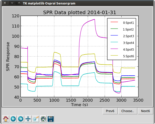
The first line imports all of the functions and data classes needed by the user. Function readicmtxt() reads an SPR data file saved by the Plexera Instrument Control Software. Other data formats are supported and described later. A object of the class Biosensor_array (BA) is created named ba1 containing the data.

Function linegraph() plots the data as a sensorgram–the SPR signal versus time. This plot appears in a separate window. At the lower left corner of the window are buttons for zooming, copying, and saving (PNG format). These buttons will be familiar to matplotlib users. At the lower right corner are three buttons for changing which ROIs are displayed. While it is possible to display all ROIs in a BA object, a plot with 25 ROIs would be too cluttered. By default, only the first six ROIs in the BA are shown. Clicking the “Next6” button will change the plot to display ROIs 6-11 and a subsequent click on the “Prev6” button will display ROIs 0-5 again. An arbitrary list of ROIs can be specified by clicking the “Choose...” button. The window must be closed in order to continue the execution of Osparai commands

Calibration and background subtraction

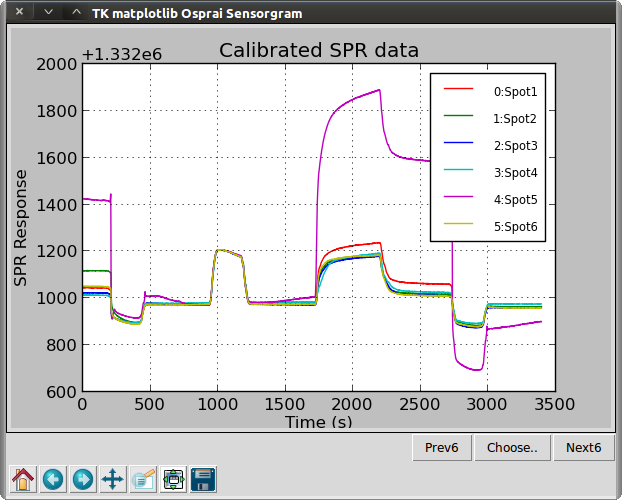
Data produced by a biosensing instrument can be reported as angle shift, reflectance, wavelength shift, resonance units (RU), or other units. This data can come from a single surface or channel, in which case the bulk refractive index changes of the samples and washes can be seen, or it may be the difference between two surfaces or channels. The example file used here is uncalibrated and unreferenced. Enter the following commands for calibration and referencing.

>>> ba2 = osp.calibrate(ba1, ba1, 950, 1050, 1333000, 1333200)
>>> osp.linegraph(ba2, "Calibrated SPR data")

>>> osp.bgset(ba2, 11)
>>> ba3 = osp.bgsubt(ba2)
>>> osp.linegraph(ba3, "Referenced SPR Data")

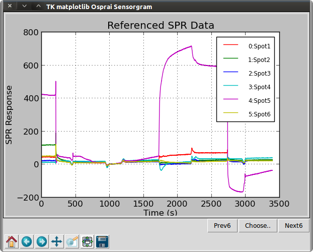
Function calibrate() uses the data in ba1 to calibrate the data in ba1 and place it in a new object ba2. The two-point calibration uses the time points (t1,t2) where the refractive indices (n1,n2) are known. In this case, we use t1=950s with n1=1333000 μRIU, and t2=1050 with n2=1333200. Function bgset() is used to specify one ROI as the reference for all ROIs in the ba object. In this case, ROI number 11 is used. No data is affected by this step. To apply background subtraction, we call the bgsubt() function. This creates a new object ba3. Next, we will arrange the sensorgrams in a more compact presentation.

>>> ba4 = osp.copyinterval(ba3, 900, 3400)
>>> osp.zerotime(ba4)
>>> osp.zerovalue(ba4)
>>> osp.linegraph(ba4, "Zeroed SPR data")

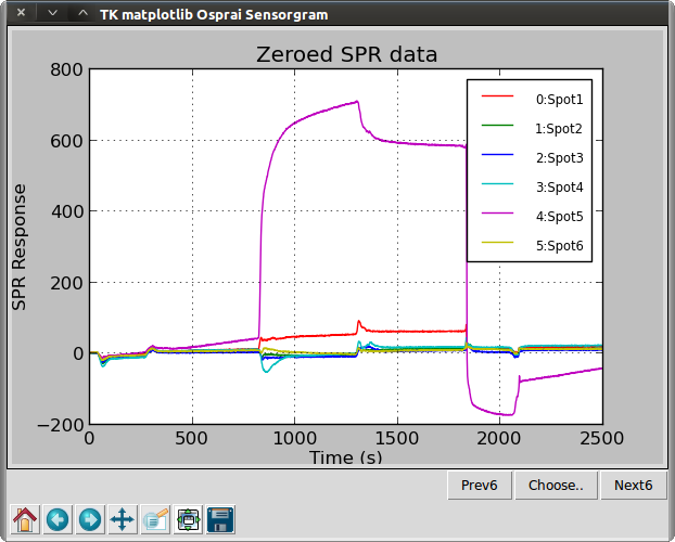
The copyinterval() function is used to create a BA object from a slice of a larger BA object. Here, unnecessary data is trimmed from the ends by selecting the time interval from 900 to 3400 seconds. The zerotime() and the zerovalue() functions are used to shift the origins of the sensorgrams to the origin of the plot.

Data simulation

Now we will create some simulated sensorgrams using a simple 1:1 interaction model. The model is defined by the built-in function osp.simple1to1() that takes nine parameters. The temporal parameters are the beginning of the experiment t0, the injection start time t1, the wash start time t2, the end of the experiment t3, all given in units of seconds. Kinetic association and dissociation are described by the on-rate kon in units of M^-1s^-1 and the off-rate koff in units of s^-1. The maximum response is described by rmax in refractive index units. Concentration is specified with conc in molar units and also by a unitless concentration factor cofa. For example, three injections of a 1:3 dilution series prepare from 1 µM may be expressed as concentrations of 1.00e-5, 3.33e-6, and 1.11e-6, all with a concentration factor of 1.0, or alternatively as a concentration of 1.0e-5 with concentration factors of 1.00, 0.33, and 0.11. Often the latter form is more convenient.

These parameters are stored using Python dictionaries—specifically, a dictionary of dictionaries. The nine parameter names are entered as keys to the top dictionary. Each parameter itself is a dictionary with four keys: value, min, max, and fixed. When curve-fitting, one or more parameters are adjusted by setting fixed='float' and the parameter’s value is constrained to remain between min and max. Here, we create a dictionary dpar and fill it with default parameters.

>>> dpar = {}
>>> dpar['t0'] = dict(value=0.0, min=0.0, max=0.0, fixed='fixed')
>>> dpar['t1'] = dict(value=30.0, min=30.0, max=30.0, fixed='fixed')
>>> dpar['rmax'] = dict(value=100.0, min=1.0, max=1000.0, fixed='fixed')
>>> dpar['conc'] = dict(value=1e-5, min=1e-12, max=1e1, fixed='fixed')
>>> dpar['cofa'] = dict(value=1.0, min=1e-10, max=1e10, fixed='fixed')
>>> dpar['kon'] = dict(value=2.1e4, min=1e1, max=1e10, fixed='fixed')
>>> dpar['t2'] = dict(value=150.0, min=150.0, max=150.0, fixed='fixed')
>>> dpar['koff'] = dict(value=1e-2, min=1e-5, max=1e-1, fixed='fixed')
>>> dpar['t3'] = dict(value=270.0, min=270.0, max=270.0, fixed='fixed')
>>> print sorted(dpar)
['cofa', 'conc', 'koff', 'kon', 'rmax', 't0', 't1', 't2', 't3']

Next, we create a biosensor array object with three sensorgrams, or regions-of-interest (roi). For each roi, we initialize the sensorgrams with 300 seconds of zeros, specify the model, and copy default parameters from dpar. We then change the concentration factors to simulate a dilution series. Finally, we perform simulations by calling the model() with the specified parameters.

>>> ba1 = osp.BiosensorArray(3,300)
>>> for roi in ba1.roi:
...     roi.time = osp.arange(300, dtype=float)  ## Samples every 1 second.
...     roi.value = osp.zeros(300, dtype=float) + 20  ## Baseline signal is 20 units.
...     roi.model = osp.simple1to1
...     roi.params = osp.deepcopy(dpar)
>>> ba1.roi[0].params['cofa']['value'] = 1.0 / 27
>>> ba1.roi[1].params['cofa']['value'] = 1.0 / 9
>>> ba1.roi[2].params['cofa']['value'] = 1.0 / 3
>>> for roi in ba1.roi:
...     roi.value = roi.model(roi.time, roi.value, roi.params)
>>> osp.dotgraph(ba1, "Simulation")

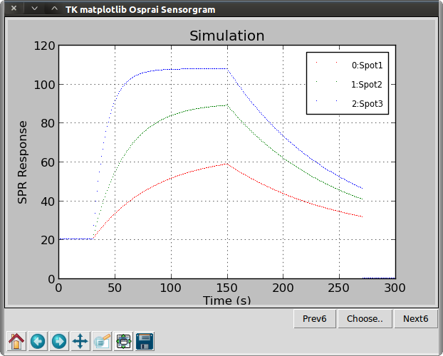
Function dotgraph() is like linegraph() but with dotted data points instead of continuous lines. We see three curves representing injections of the same analyte at concentrations of 1.11 (red), 3.33 (green), and 10 µM (blue).

Curve-fitting

Osprai uses a modified version of the Levenberg-Marquardt least-squares algorithm (LMA) for fitting parameters. The function mcmla() provides LMA fitting on multiple curves with constrained parameters. The use of constraints can improve speed and eliminate nonsensical solutions such as negative values for binding kinetic rate parameters. In this example, we constrain the rmax parameter to deliberately produce incorrect kon and koff parameter results.

>>> ba1.roi[0].params['rmax'] = {'value':10.0, 'min':1.0, 'max':80.0, 'fixed':'float'}
>>> ba1.roi[0].params['kon']['fixed'] = 'float'
>>> ba1.roi[0].params['koff']['fixed'] = 'float'
>>> ba1.roi[1].params['rmax']['fixed'] = 0
>>> ba1.roi[1].params['kon']['fixed'] = 0
>>> ba1.roi[1].params['koff']['fixed'] = 0
>>> ba1.roi[2].params['rmax']['fixed'] = 0
>>> ba1.roi[2].params['kon']['fixed'] = 0
>>> ba1.roi[2].params['koff']['fixed'] = 0

We specify which parameters we wish to solve for by changing their ‘fixed’ key from ‘fixed’ to ‘float’. All three ROIs in this BA have the same model and the same parameters, so we only set the parameters in one of the ROIs to ‘float’. Here, we choose the the first ROI, roi[0], and change ‘fixed’ to ‘float’ for ‘rmax’, ‘kon’, and ‘koff’ parameters. In addition, we specify that ‘rmax’ will have a ‘max’ value of 80.0. Next, we specify that the ‘rmax’, ‘kon’, and ‘koff’ values for roi[1] and roi[2] are the same as for roi[0]. We do this by setting their ‘fixed’ key to 0, a reference to roi[0]. Now we are ready to start curve-fitting.

>>> osp.mclma(ba1.roi)
0 koff 0.0100 kon 21000.0000 rmax 10.0000 1 2 ssq 1523066.7
0 koff 0.0100 kon 21000.0000 rmax 10.0000 1 2 ssq ...

>>> print round(ba1.roi[0].params['kon']['value'])
29679.0
>>> osp.dualgraph(ba1, ba1, "Fitting with an incorrect rmax constraint")

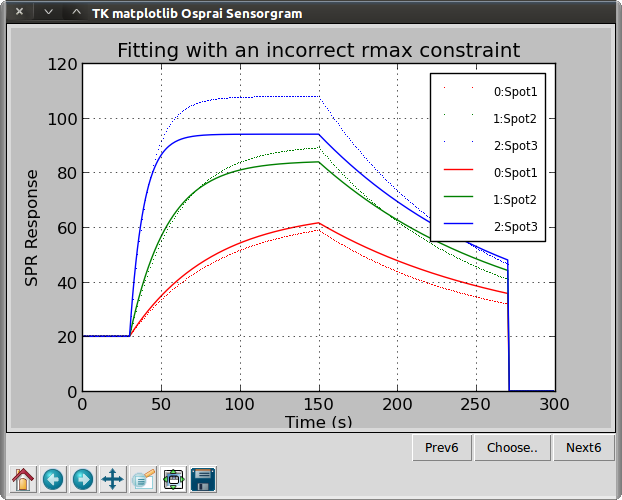
We call the curve-fitting function with mclma(ba2.roi) This function will print out the values of the floating parameters and the sum-squared error after each iteration. After about 30 iterations, in this case, the algorithm converges upon a solution. Since ‘rmax’ was constrained to 80.0, with the real ‘rmax’ is 100.0, the resulting best-fit kon is found to be high (28000 vs. 20000).

We use the dualgraph() function to display two biosensor array data sets, the first with dotted lines and the second with solid lines. If the same object is specified for both data sets, as in this example, the actual sensorgram is plotted with dotted lines while the fitted data is plotted with solid lines. Next, we will loosen the rmax constraint and look at the effect of noise.

>>> ba1.roi[0].params['rmax']['max'] = 1000
>>> mynoise = dict(rms=dict(value=1.5))
>>> for roi in ba1.roi:
...     roi.value = osp.noise(roi.time, roi.value, mynoise)
>>> osp.mclma(ba1.roi)
0 koff 0.0081 kon 29678.8440 rmax 80.0000 1 2 ssq ...

>>> print round(ba1.roi[0].params['kon']['value'])
2...
>>> osp.dualgraph(ba1, ba1, "Best fit")

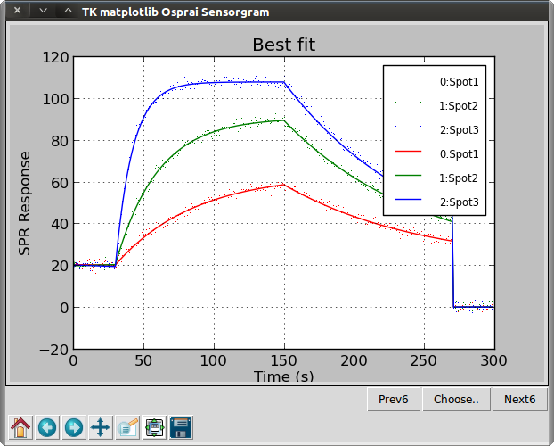
We have increased the rmax to a value far higher than the actual value. We only need to change roi[0] as the other two are tied to it. Next, we add some white noise to the sensorgrams using the noise() data model and re-run the curve-fitting algorithm. This time, we obtain kinetics very close to the expected values.

File format conversion

Functions are provided to read and write several Biacore and Plexera file formats. Optionally, microarray annotations can be added to the SPR data from GAL or Key files. These annotations are saved when data files are written, if the file format provides support. Examples are given below:

>>> osp.writebiosensor(ba1, "testbiosensor.txt")
File testbiosensor.txt saved in ...
>>> ba2 = osp.readbiosensor("testbiosensor.txt")
This Biosensor file has 300 datapoints for 3 ROIs.
>>>
>>> osp.writeclamp(ba1, "testclamp.txt")
File testclamp.txt saved in ...
>>>
>>> osp.writesprit(ba1, "testsprit.txt")
File testsprit.txt saved in ...
>>> ba2 = osp.readsprit("testsprit.txt")
Successfully loaded information for 3 ROIs.

Online help

The Python help() function can be used at any time to display the online documentation for all Osprai functions and classes.

>>> import osprai_one as osp
>>> help(osp)
Help on module osprai_one:...

NAME
   osprai_one

FILE
   ( ..many pages follow.. )

>>> help(osp.linegraph)
Help on function linegraph in module vu_module:...

linegraph(baLine, title='')
     Display signal vs time using continuous lines.

     :param baLine: Object containing the data.
     :type baLine: ba_class
     :param title: Title to place above the graph.
     :type title: str
     :returns: nothing