Table of Contents
CMView is an interactive Contact Map viewer for protein structures. CMView will allow you to display the contact map and interact with it as well as to show features of the contact map in the corresponding 3-dimensional structure by using the PyMol molecular viewer.
The first step to get your contact map on screen is to load it by using from the menu. Here there are many options for the source of your data:
-
which will download the PDB data for your chosen 4 letter PDB code directly from the Protein Data Bank's web
-
, if what you have is a model output of a molecular modeling program in PDB format, then choose this option to load your data
-
, to load CASP residue-residue contact predictions. You can also save files with this format with ->
-
refers to CMView's own format, you can choose this if you previously saved a file from CMView in this format.
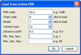
For this example we will load from Online PDB the PDB entry 1bxy, with chain code A. In the load dialog we can then choose the contact type and distance cutoff, we take Ca (for C-alpha) and 8.0 Ã… as cutoff:
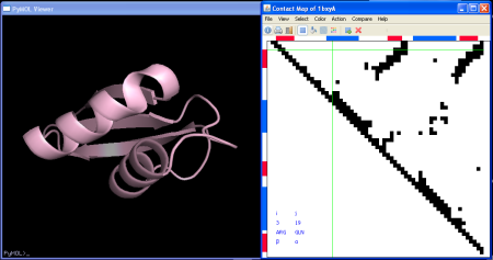
After clicking OK the contact map is displayed and the 3D structure is loaded to the PyMol molecular viewer:
Some useful things you can do once your contact map has been loaded are:
-
Select contacts: rectangle select, fill select, diagonal select. While on diagonal mode the sequence separation will be shown together with the coordinates in the lower left corner.
-
Show the distance map overlaid ( menu). You can still select contacts while the distance map is shown
-
Click on the Info
 button to get a full report on the contact map:
number of contacts, sequence etc.
button to get a full report on the contact map:
number of contacts, sequence etc. -
The top and left rulers show the color coded secondary structure elements: blue for alpha-helix, red for beta-sheet, green for turns. You can select contacts between 2 secondary structure elements by clicking on the first element in the top ruler and then on the second element on the left ruler. You will get something like:
-
Some other useful selections for secondary structure elements can also be done from the menu: helix-helix contacts, strand-strand and intra/inter secondary structure elements (SSEs) contacts.
-
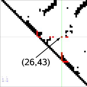
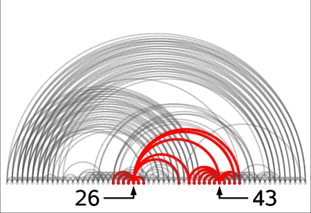
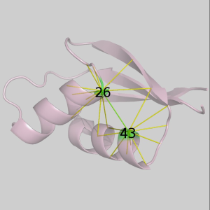
Select neighborhoods, i.e. all the contacts for a given residue. Just choose the and click on the ruler: all neighbors of the chosen residue will be selected. If you click instead on the contact map you will get the neighbors for the 2 residues of the clicked residue pair. For instance if you click on cell (26,43) one gets all neighbors of residue 26 and all neighbors of residue 43. Here we present this in the contact map view, in a graph representation and in the 3-dimensional structure:
At any time while navigating around the contact map or the residue rulers you will always be able to see the contact map coordinates of the current contact or residue: residue number, residue type and secondary structure. You can also view the original author assigned PDB residue numbers if you switch the appropriate option on in the menu (only if structure was loaded from Online PDB).
Remember in all selections above, you can always use CTRL+click to add to the current selection.
Here is where CMView becomes most useful: the visualization of 2D elements in the 3D structure. After selecting residue/contacts in the contact map we can then view their correspondence on the 3-dimensional protein structure by using the PyMol molecular viewer. Commands are sent directly and interactively to PyMol. There are two functions:
-
will show the selected contacts as distance objects between the C-alpha atoms of the 2 residues part of the contact. As well as the distance object a selection is created in PyMol which contains all residues present in the contact selection, useful for further manipulations in PyMol.
-
(available from the context menu) will show the distance between the current (where you right-clicked) pair of residues as a distance object in PyMol.
As an example here we show contacts between secondary structures element for our structure 1bxy. Corresponding to each function in the Select menu we have:
helix-helix contacts,
strand-strand contacts,
contacts within SS elements
and finally contacts between SS elements
Of course PyMol still works as usual so that it is possible to do other things with the selections: highlighting or showing different representations like sticks, spheres etc.
As an interesting example for the contact map comparison feature we will use a CASP7 prediction to see what predictions get right or not in terms of contacts. We want to compare the native structure of target T0354 to a prediction. So first we load the reference structure from the PDB file (same procedure as before) and then the prediction by using -> -> . As before we choose contact type Ca and 8.0 Ã… distance cutoff.
After pressing OK the second contact map is calculated and a dialog comes up to choose what type of alignment we want:
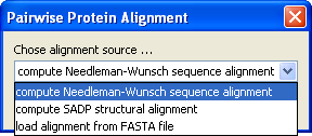
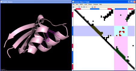
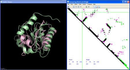
For this case we have two structures with the same sequence so we can simply select Needleman-Wunsch which will do the trivial alignment. The second contact map is displayed and at the same time the corresponding structure is loaded to PyMol superimposed to the first structure:
CMView offers here also a structural alignment (SADP) based on maximum contact map overlap that would be useful when we want to compare distantly related sequences. See CMView's full reference for more info about SADP. As a last alternative you can also load your own alignment from a FASTA file.
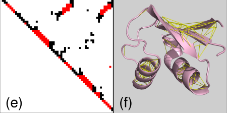
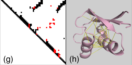
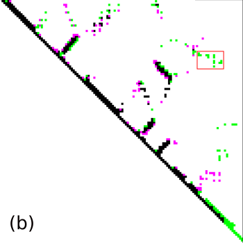
The pairwise comparison mode shows the two contact maps with contacts in 3 colors:
-
black for common contacts
-
pink for contacts unique to the first structure (the real structure)
-
green for contacts unique to the second structure (the prediction)
For our example of prediction against real this allows us to see at a glance over-predicted (pink) and under-predicted contacts (green).
It is possible to switch between displaying each of
the sets with the toggle buttons


 in the
tool bar. Selections always refer to the currently
displayed set.
in the
tool bar. Selections always refer to the currently
displayed set.
As in single mode above, the coordinates are displayed
in the lower left corner this time for the two
structures. The Info function
will also display now information for both structures
including the numbers of common contacts and unique
contacts to each structure.
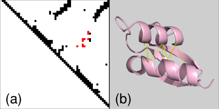
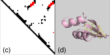
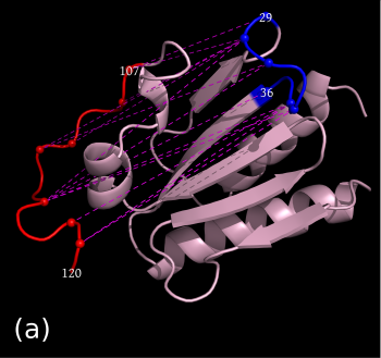
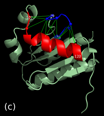
Finally as before we can also interactively send contacts to PyMol. In the pairwise case it gets more interesting because we get a clear comparison of contacts made/not made by the two structures. We will get now yellow edges in both structures for the common contacts, pink edges for the contacts only in the first structure and green edges for contacts only in the second structure. Correspondingly dashed pink/green edges will be displayed representing the absent (not-made) contacts in the opposite structures.
As an example we select the green contacts within the red rectangle in b) below. For clarity we have separated the two structures and highlighted residues with colors and spheres in PyMol: c) contacts present in the second structure with solid green edges, a) matching (from alignment) contacts absent in the second structure, dashed pink edges.
Two extra functions are available in the pairwise comparison mode:
-
will superimpose the two structures in PyMol doing a best fit of residues from the selected contacts.
-
will show the alignment matching pairs for the contacts selected.